library(haldensify)
library(plotly) # for interactive plotsEstimating conditional densities using HAL
In this example, we demonstrate one possible way to estimate conditional densities using HAL through the pooled logistic regression.
Problem setup
We observe \(n\) i.i.d. copies of \(O=(X,T)\sim P_0\in\mathcal{M}\), where
\(X \in \mathbb{R}^d\) are covariates;
\(T \in \mathbb{R}\) is a continuous variable.
Our target is the conditional density \(p_0(t \mid X)\).
Pooled logistic regression for estimating conditional densities
One way to estimate the conditional density of \(T\), given \(X\) using HAL is through discretizing \(T\). This technique has been considered in Diáz and van der Laan (2011). In practice, this can be implemented via a pooled logistic regression. Specifically, consider a set of \(k\) bins \(\{[t_{j-1},t_j):j=1,\dots,k\}\) formed by \(t_0,\dots,t_k\) that partitions \(T\). Now, we parameterize the conditional density in terms of discrete hazards for each bin. Let \(\tilde{\lambda}_j(X)=P(T\in[t_{j-1},t_j)\mid T\geq t_{j-1},X)\), that is, \(\tilde{\lambda}_j\) is the discrete hazard of falling into bin \(j\), given having “survived” up to \(t_{j-1}\). Then, we have that: \[ P(T\in[t_{j-1},t_j)\mid X)=\tilde{\lambda}_j(X)\prod_{m=1}^{j-1}(1-\tilde{\lambda}_m(X)). \] The conditional density can then be obtained as \[ p(t\mid X)=\sum_{j=1}^k \frac{P(T\in[t_{j-1},t_j)\mid X)}{t_j-t_{j-1}}I(t\in[t_{j-1},t_j)). \] For \(n\) independent units, the likelihood corresponds to the likelihood of an indicator in a repeated measures data set, where the outcome is an indicator of whether \(T_i\) falls within a specific bin, i.e., \(T_i\in(t_{\alpha-1},t_\alpha]\). For each subject, observations are repeated as many times as there are bins \([t_{\alpha-1},t_\alpha)\) prior to the bin in which \(T_i\) lies in. One could then run a logistic regression with, for example, zero-order HAL basis, on this repeated data set to obtain the estimated bin-level conditional densities. Finally, a piecewise constant conditional density function over \(\mathbb{R}\) can be obtained by normalizing each bin-level estimate by the corresponding bin width.
Once we have mapped the discrete conditional density into a conditional density, we can use cross-validation based on the log-likelihood loss to select the number of bins \(k\).
Load required packages
We first load the required packages.
The package implements the nonparametric conditional density estimation via pooled logistic regressions using HAL, as discussed above .
Data generating process
Let’s consider a setting where we are tasked to estimate the generalized propensity score (conditional density of a continuous treatment given covariates). This task could arise in the context of, for example, estimating the effect of a stochastic intervention on a continuous treatment. Suppose researchers collect two baseline covariates \(W_1\) and \(W_2\), each following a standard normal distribution. Suppose the treatment \(A\) is a continuous variable following a normal distribution with a mean given by \(1+0.3W_1-1.5W_2\). To introduce some heteroskedasticity, we set its standard deviation to \(2+0.3|W1|\).
set.seed(75681)
data <- read.csv("data/data_cde.csv")
Use the haldensify function to estimate the conditional density of A given W
The below one liner uses the function to estimate the conditional density of \(A\) given \(W=(W_1,W_2)\) using zero-order HAL basis functions. The function automatically selects the number of bins via cross-validation based on the log-likelihood loss.
haldensify_fit <- haldensify(A = data$A,
                             W = data$W,
                             lambda_seq = exp(seq(-0.1, -10, length = 300)))
Let’s plot the empirical risk (negative log-likelihood) as a function of the regularization parameter \(\lambda\).
# empirical risk vs. lambda
risk_vs_lambda <- plot(haldensify_fit)
risk_vs_lambda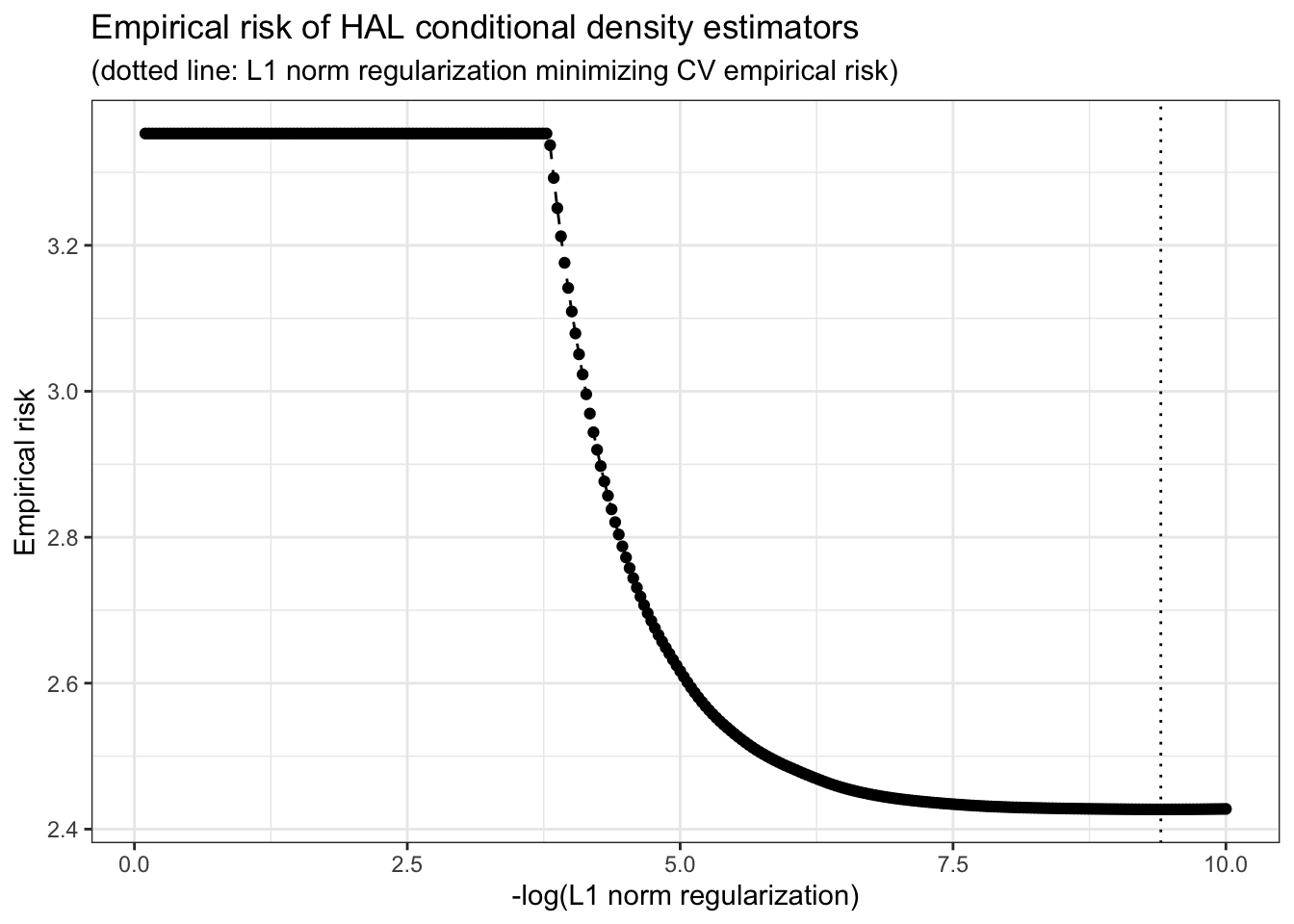
Plot the estimated conditional density
Now, let’s visualize the estimated conditional density of \(A\) at \(W_2=0\) over a grid of \(W_1\) values, and compare it with the true conditional density.
# compute true conditional densities over a grid
source("data/sim_data_cde.R")
n <- 2000
W1_vals <- seq(-2, 2, length.out = 20)
W2_fixed <- 0
A_vals <- seq(-2, 6, length.out = 30)
grid <- expand.grid(W1 = W1_vals,
                    W2 = W2_fixed,
                    A = A_vals)
grid$true_dens <- sim_data_cde(n, grid = grid)$A
grid$pred_dens <- predict(haldensify_fit,
                          new_A = grid$A,
                          new_W = grid[, c("W1", "W2")])
pred_dens_mat <- matrix(grid$pred_dens,
                        nrow = length(A_vals),
                        ncol = length(W1_vals),
                        byrow = FALSE)
true_dens_mat <- matrix(grid$true_dens,
                        nrow = length(A_vals),
                        ncol = length(W1_vals),
                        byrow = FALSE)

plt_pred <- plot_ly(x = A_vals, y = W1_vals, z = pred_dens_mat,
        colorscale = "Greens") %>%
  add_surface() %>%
  layout(title = list(text = "Estimated Conditional Density",
                      font = list(size = 18, color = "black"),
                      yref = "container",
                      y = 0.98),
         scene = list(xaxis = list(title = "A", titlefont = list(size = 14)),
                      yaxis = list(title = "W1", titlefont = list(size = 14)),
                      zaxis = list(title = "Density",
                                   titlefont = list(size = 14),
                                   range = c(0, 0.2)),
                      camera = list(eye = list(x = 1.5, y = 1.5, z = 1))),
         legend = list(x = 0.8, y = 1, font = list(size = 12)))

plt_true <- plot_ly(x = A_vals, y = W1_vals, z = true_dens_mat,
        colorscale = "Reds") %>%
  add_surface() %>%
  layout(title = list(text = "True Conditional Density",
                      font = list(size = 18, color = "black"),
                      yref = "container",
                      y = 0.98),
         scene = list(xaxis = list(title = "A", titlefont = list(size = 14)),
                      yaxis = list(title = "W1", titlefont = list(size = 14)),
                      zaxis = list(title = "Density",
                                   titlefont = list(size = 14),
                                   range = c(0, 0.2)),
                      camera = list(eye = list(x = 1.5, y = 1.5, z = 1))),
         legend = list(x = 0.8, y = 1, font = list(size = 12)))
# plot the estimated conditional density
plt_pred
# plot the true conditional density
plt_true