library(atmle) # not on CRAN yet; install from GitHub
library(sl3)
library(origami)
library(purrr)
library(ggplot2)
options(sl3.verbose = FALSE)Analyzing Hybrid RCTs with Adaptive-TMLE
Introduction
In this coding example, we demonstrate through a synthetic example of how to use Adaptive-TMLE to improve the efficiency of treatment effect estimators of a non-inferiority randomized controlled trial (RCT) by augmenting it with external patient-level real-world data (RWD) to establish treatment effect superiority.
Problem setup
Suppose we observe \(n\) copies of the random variable \(O=(S,W,A,Y)\) sampled i.i.d from a probability distribution \(P_0\) from a statistical model \(\mathcal{M}\). Here, \(S\in\{0,1\}\) indicates whether the patient belongs to the RCT; \(W\in\mathbb{R}^d\) represents a set of baseline covariates; \(A\in\{0,1\}\) denotes treatment assignment; and \(Y\in\mathbb{R}\) is the clinical outcome of interest. We consider a setting where both the RCT and external data include treatment and control arms.
Estimand
We define the following target estimand: \[ \Psi(P)=E_{P_W}[E_P(Y_1-Y_0\mid S=1,W)], \] which represents the treatment effect within the trial, averaged over the pooled covariate distribution, where \(P_W\) is the distribution of \(W\) in the pooled population. Identification of this estimand requires the following assumptions:
A1: \((Y_0,Y_1)\perp A\mid S=1,W\) (mean exchangeability in the RCT);
A2: \(0<P(A=1\mid S=1,W)<1\) (positivity of treatment assignment in the RCT);
A3: \(P(S=1\mid W)>0\) (positivity of trial participation in the pooled population).
Assumptions A1 and A2 hold under a well-designed RCT. Assumption A3 requires that for every covariate stratum in the pooled population, there is a non-zero probability of trial participation. This assumption may be violated if the RCT has strict eligibility criteria that exclude certain patient subgroups present in the RWD. To make this assumption more plausible, one could consider apply the same eligibility criteria to select the RWD as those used in the RCT.
Under A1–A3, the estimand is identified as \[ \Psi(P_0)=E_0[E_0(Y\mid S=1,W,A=1)-E_0(Y\mid S=1,W,A=0)]. \]
Decomposition of the target estimand
Note that we can express our target estimand: \[ \Psi(P_0)=E_0[E_0(Y\mid S=1,W,A=1)-E_0(Y\mid S=1,W,A=0)] \] as a difference of two other estimands, the pooled-ATE estimand \[ \tilde{\Psi}(P_0)=E_0[E_0(Y\mid W,A=1)-E_0(Y\mid W,A=0)] \] and the bias estimand: \[ \begin{align*} \Psi^\#(P_0)&\equiv\tilde{\Psi}(P_0)-\Psi(P_0)\\ \Psi(P_0)&=\tilde{\Psi}(P_0)-\color{red}{\Psi^\#(P_0)} \end{align*} \] That is, we can view our target estimand as a bias-corrected version of the pooled-ATE estimand \(\tilde{\Psi}\). The bias term \(\Psi^\#\) quantifies any kind of bias that resulted in differences between the pooled-ATE and the ATE in the RCT, including bias due to unmeasured confounding in the external data, and bias due to different adherence patterns between the RCT and external real-world environment.
With some algebra, the bias estimand could be written as \[
\Psi^\#(P_0)=E[\Pi(0\mid W,0)\tau_S(W,0)-\Pi(0\mid W,1)\tau_S(W,1)],
\] where \[
\begin{align*}
\Pi(s\mid W,A)&=P(S=s\mid W,A),\\
\tau_S(W,A)&=E(Y\mid S=1,W,A)-E(Y\mid S=0,W,A).
\end{align*}
\] In our coding exercise, we will learn to use A-TMLE from the atmle R package to estimate \(\tilde{\Psi}\) and \(\Psi^\#\), respectively.
Loading required packages
We first load the required packages:
Data summary
seed <- 113
data <- read.csv("data/data_atmle.csv")
head(data)
W1 W2 W3 W4 S A Y
1 -0.02869571 -0.4045813 1 0.06485454 0 0 -0.07675618
2 -0.57147442 -1.5312715 1 -0.09930300 1 0 1.82348172
3 0.84844646 -1.1060846 1 -0.97265865 1 1 3.26502543
4 -0.19345784 1.5640041 0 0.99635468 1 1 -1.57223734
5 1.48350181 0.6554029 0 -0.39934316 0 1 1.28774759
6 1.83544940 0.1132685 1 1.23493999 1 0 3.71633853Candidate estimators
We will compare the standard TMLE estimator with the A-TMLE estimator side-by-side.
A standard TMLE estimator
The canonical gradient of \(\Psi\) at \(P\) in a nonparametric model is given by \[
\begin{align*}
D_{\Psi,P}&=Q_P(1,W,1)-Q_P(1,W,0)-\Psi(P)\\
&+\frac{S}{P(S=1\mid W)}\cdot\frac{2A-1}{g_P(A\mid 1,W)}(Y-Q_P(S,W,A)),
\end{align*}
\] where \(Q_P(S,W,A)\equiv E_P(Y\mid S,W,A)\) and \(g_P(A\mid S,W)\equiv P(A\mid S,W)\). Therefore, one could construct a standard TMLE estimator with clever covariate \[
\frac{S}{P(S=1\mid W)}\cdot\frac{2A-1}{g_P(A\mid 1,W)}.
\] This TMLE is implemented in the nonparametric() function in the atmle R package:
sl_lib <- list(Lrnr_glm$new(),
               Lrnr_dbarts$new(),
               Lrnr_xgboost$new())
set.seed(seed)
tmle_res <- nonparametric(data = data,
                          S = "S",
                          W = c("W1", "W2", "W3", "W4"),
                          A = "A",
                          Y = "Y",
                          family = "gaussian",
                          Pi_method = sl_lib,
                          g_method = "glm",
                          Q_method = sl_lib,
                          Q_pooling = TRUE,
                          v_folds = 5)
Adaptive-TMLE estimator
set.seed(seed)
atmle_res <- atmle(data = data,
                   S = "S",
                   W = c("W1", "W2", "W3", "W4"),
                   A = "A",
                   Y = "Y",
                   family = "gaussian",
                   theta_method = sl_lib,
                   Pi_method = sl_lib,
                   g_method = sl_lib,
                   theta_tilde_method = sl_lib,
                   bias_working_model = "HAL",
                   pooled_working_model = "HAL",
                   target_method = "oneshot",
                   enumerate_basis_args = list(max_degree = 3,
                                               smoothness_orders = 1),
                   v_folds = 5)
learning θ(W,A)=E(Y|W,A)...Done!
learning g(1|W)=P(A=1|W)...Done!
learning Π(S=1|W,A)=P(S=1|W,A)...Done!
learning τ(W,A)=E(Y|S=1,W,A)-E(Y|S=0,W,A)...Done!
[1] -0.002126372
learning θ̃(W)=E(Y|W)...Done!
learning Τ(W)=E(Y|W,A=1)-E(Y|W,A=0)...Done!
targeting beta_A...Done!
Pooled ATE: 0.75524 (0.53173, 0.97874)
Bias: 0.46795 (0.27789, 0.658)
Bias-corrected ATE: 0.28729 (0.014865, 0.55972)Let’s study the output of it a bit more closely.
First, let’s examine the point estimates. The pooled ATE estimate is 0.76, while the bias-correct ATE estimate is 0.29 We also see that the estimate of the bias is 0.47 Indeed, the bias correction is pushing us closer to the truth, which is 0.30.
df_plot <- data.frame(Estimator = c("Standard TMLE",
                                    "Pooled-ATE",
                                    "Bias-corrected ATE (A-TMLE)"),
                      Estimate = c(tmle_res$psi_pooled_W,
                                   atmle_res$psi_tilde_est,
                                   atmle_res$est),
                      Lower = c(tmle_res$lower_pooled_W,
                                atmle_res$psi_tilde_lower,
                                atmle_res$lower),
                      Upper = c(tmle_res$upper_pooled_W,
                                atmle_res$psi_tilde_upper,
                                atmle_res$upper))
df_plot$Estimator <- factor(df_plot$Estimator,
                            levels = c("Standard TMLE",
                                       "Bias-corrected ATE (A-TMLE)",
                                       "Pooled-ATE"))
ggplot(df_plot, aes(x = Estimator, y = Estimate, fill = Estimator)) +
  geom_point() +
  geom_errorbar(aes(ymin = Lower, ymax = Upper), width = 0.2, size = 0.8) +
  geom_hline(yintercept = 0.2998021, linetype = "dashed", color = "red") +
  geom_hline(yintercept = 0, linetype = "dashed", color = "gray") +
  theme_minimal(base_size = 13) +
  labs(title = "Point Estimates with 95% Confidence Intervals",
       y = "Estimate",
       x = "") +
  theme(legend.position = "none",
        plot.title = element_text(hjust = 0.5)) +
  coord_flip()
Warning: Using `size` aesthetic for lines was deprecated in ggplot2 3.4.0.
ℹ Please use `linewidth` instead.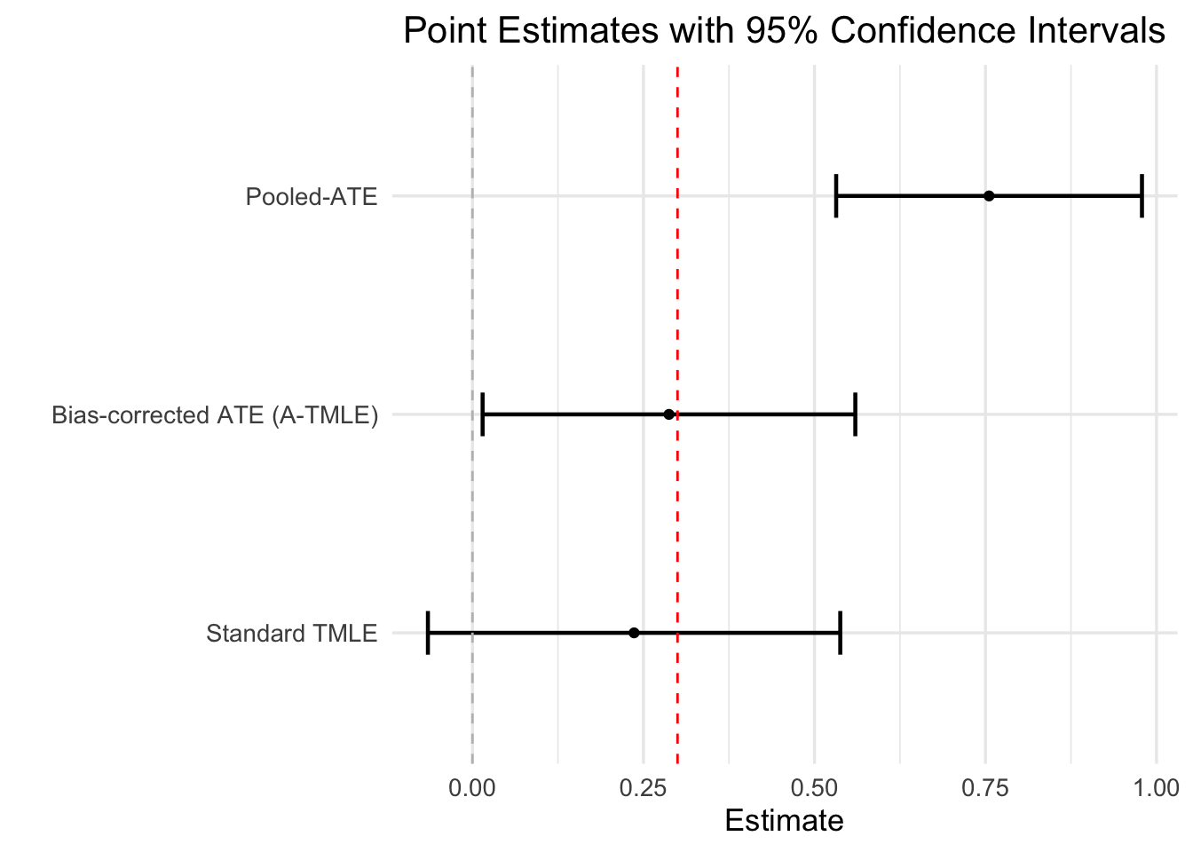
Let’s also compare the widths of the 95% confidence intervals:
ci_width_tmle <- tmle_res$upper_pooled_W-tmle_res$lower_pooled_W
ci_width_atmle <- atmle_res$upper-atmle_res$lower
round(ci_width_atmle/ci_width_tmle, 3)
[1] 0.904The width of the 95% confidence interval of the A-TMLE estimator is about 90% of that of the standard TMLE estimator.
References
Mark van der Laan, Sky Qiu & Lars van der Laan (2024). Adaptive-TMLE for the Average Treatment Effect based on Randomized Controlled Trial Augmented with Real-World Data. In press at Journal of Causal inference. [Paper]
Sky Qiu, Jens Tarp, Andrew Mertens & Mark van der Laan (2025). An Estimator-Robust Design for Augmenting Randomized Controlled Trial with External Real-World Data. arXiv preprint. [Paper]